Core Concepts
This page introduces the fundamental concepts of flixOpt through practical scenarios. Understanding these concepts will help you model any system involving flows and conversions.
The Big Picture
Imagine you're managing a district heating system. You have:
- A gas boiler that burns natural gas to produce heat
- A heat pump that uses electricity to extract heat from the environment
- A thermal storage tank to buffer heat production and demand
- Buildings that need heat throughout the day
- Access to the gas grid and electricity grid
Your goal: minimize total operating costs while meeting all heat demands.
This is exactly the kind of problem flixOpt solves. Let's see how each concept maps to this scenario.
Buses: Where Things Connect
A Bus is a connection point where energy or material flows meet. Think of it as a junction or hub.
In our heating system
- Heat Bus — where heat from the boiler, heat pump, and storage meets the building demand
- Gas Bus — connection to the gas grid
- Electricity Bus — connection to the power grid
The key rule: At every bus, inputs must equal outputs at each timestep.
This balance constraint is what makes your model physically meaningful — energy can't appear or disappear.
Carriers
Buses can be assigned a carrier — a type of energy or material (electricity, heat, gas, etc.). Carriers enable automatic coloring in plots and help organize your system semantically:
heat_bus = fx.Bus('HeatNetwork', carrier='heat')  # Uses default heat color
elec_bus = fx.Bus('Grid', carrier='electricity')
See Color Management for details.
Flows: What Moves Between Elements
A Flow represents the movement of energy or material. Every flow connects a component to a bus, with a defined direction.
In our heating system
- Heat flowing from the boiler to the Heat Bus
- Gas flowing from the Gas Bus to the boiler
- Heat flowing from the Heat Bus to the buildings
Flows have:
- A size (capacity) — "This boiler can deliver up to 500 kW"
- A flow rate — "Right now it's running at 300 kW"
Components: The Equipment
Components are the physical (or logical) elements that transform, store, or transfer flows.
Converters — Transform One Thing Into Another
A LinearConverter takes inputs and produces outputs with a defined efficiency.
In our heating system
- Gas Boiler: Gas → Heat (η = 90%)
- Heat Pump: Electricity → Heat (COP = 3.5)
The conversion relationship:
Storages — Save for Later
A Storage accumulates and releases energy or material over time.
In our heating system
- Thermal Tank: Store excess heat during cheap hours, use it during expensive hours
The storage tracks its state over time:
Sources & Sinks — System Boundaries
Sources and Sinks connect your system to the outside world.
In our heating system
- Gas Source: Buy gas from the grid at market prices
- Electricity Source: Buy power at time-varying prices
- Heat Sink: The building demand that must be met
Effects: What You're Tracking
An Effect represents any metric you want to track or optimize. One effect is your objective (what you minimize or maximize), others can be constraints.
In our heating system
- Costs (objective) — minimize total operating costs
- CO₂ Emissions (constraint) — stay below 1000 tonnes/year
- Gas Consumption (tracking) — report total gas used
Effects can be linked: "Each kg of CO₂ costs €80 in emissions trading" — this creates a connection from the CO₂ effect to the Costs effect.
FlowSystem: Putting It All Together
The FlowSystem is your complete model. It contains all buses, components, flows, and effects, plus the time definition for your optimization.
import flixopt as fx

# Define timesteps (e.g., hourly for one week)
timesteps = pd.date_range('2024-01-01', periods=168, freq='h')

# Create the system
flow_system = fx.FlowSystem(timesteps)

# Add elements
flow_system.add_elements(heat_bus, gas_bus, electricity_bus)
flow_system.add_elements(boiler, heat_pump, storage)
flow_system.add_elements(costs_effect, co2_effect)
The Workflow: Model → Optimize → Analyze
Working with flixOpt follows three steps:
graph LR
    A[1. Build FlowSystem] --> B[2. Run Optimization]
    B --> C[3. Analyze Results]
1. Build Your Model
Define your system structure, parameters, and time series data.
2. Run the Optimization
Optimize your FlowSystem with a solver:
3. Analyze Results
Access solution data directly from the FlowSystem:
# Access component solutions
boiler = flow_system.components['Boiler']
print(boiler.solution)

# Get total costs
total_costs = flow_system.solution['costs|total']

# Use statistics for aggregated data
print(flow_system.statistics.flow_hours)

# Plot results
flow_system.statistics.plot.balance('HeatBus')
Quick Reference
| Concept | What It Represents | Real-World Example |
|---|---|---|
| Bus | Connection point | Heat network, electrical grid |
| Flow | Energy/material movement | Heat delivery, gas consumption |
| LinearConverter | Transformation equipment | Boiler, heat pump, turbine |
| Storage | Time-shifting capability | Battery, thermal tank, warehouse |
| Source/Sink | System boundary | Grid connection, demand |
| Effect | Metric to track/optimize | Costs, emissions, energy use |
| FlowSystem | Complete model | Your entire system |
FlowSystem API at a Glance
The FlowSystem is the central object in flixOpt. After building your model, all operations are accessed through the FlowSystem and its accessors:
flow_system = fx.FlowSystem(timesteps)
flow_system.add_elements(...)

# Optimize
flow_system.optimize(solver)

# Access results
flow_system.solution                    # Raw xarray Dataset
flow_system.statistics.flow_hours       # Aggregated statistics
flow_system.statistics.plot.balance()   # Visualization

# Transform (returns new FlowSystem)
fs_subset = flow_system.transform.sel(time=slice(...))

# Inspect structure
flow_system.topology.plot()
Accessor Overview
| Accessor | Purpose | Key Methods |
|---|---|---|
solution | Raw optimization results | xarray Dataset with all variables |
statistics | Aggregated data | flow_rates, flow_hours, sizes, charge_states, total_effects |
statistics.plot | Visualization | balance(), heatmap(), sankey(), effects(), storage() |
transform | Create modified copies | sel(), isel(), resample(), cluster() |
topology | Network structure | plot(), start_app(), infos() |
Element Access
Access elements directly from the FlowSystem:
# Access by label
flow_system.components['Boiler']        # Get a component
flow_system.buses['Heat']               # Get a bus
flow_system.flows['Boiler(Q_th)']       # Get a flow
flow_system.effects['costs']            # Get an effect

# Element-specific solutions
flow_system.components['Boiler'].solution
flow_system.flows['Boiler(Q_th)'].solution
Beyond Energy Systems
While our example used a heating system, flixOpt works for any flow-based optimization:
| Domain | Buses | Components | Effects |
|---|---|---|---|
| District Heating | Heat, Gas, Electricity | Boilers, CHPs, Heat Pumps | Costs, CO₂ |
| Manufacturing | Raw Materials, Products | Machines, Assembly Lines | Costs, Time, Labor |
| Supply Chain | Warehouses, Locations | Transport, Storage | Costs, Distance |
| Water Networks | Reservoirs, Treatment | Pumps, Pipes | Costs, Energy |
Next Steps
- Building Models — Step-by-step guide to constructing models
- Examples — Working code for common scenarios
- Mathematical Notation — Detailed constraint formulations
Advanced: Extending with linopy
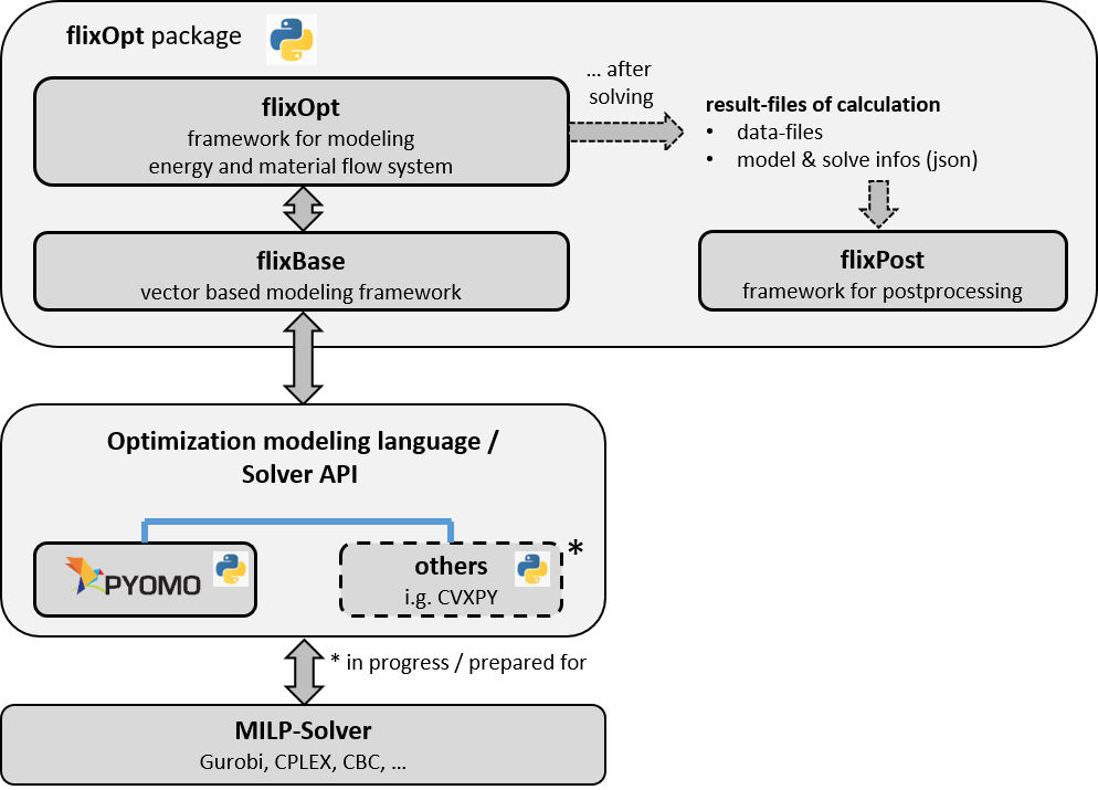
flixOpt is built on linopy. You can access and extend the underlying optimization model for custom constraints:
# Build the model (without solving)
flow_system.build_model()

# Access the linopy model
model = flow_system.model

# Add custom constraints using linopy API
model.add_constraints(...)

# Then solve
flow_system.solve(fx.solvers.HighsSolver())
This allows advanced users to add domain-specific constraints while keeping flixOpt's convenience for standard modeling.